January 1, 0001
library(tidyr)
library(ggplot2)
library(dplyr)
##
## Attaching package: 'dplyr'## The following objects are masked from 'package:stats':
##
## filter, lag## The following objects are masked from 'package:base':
##
## intersect, setdiff, setequal, unionlibrary(tibble)
library(MASS)##
## Attaching package: 'MASS'## The following object is masked from 'package:dplyr':
##
## selectlibrary(lmtest)## Loading required package: zoo##
## Attaching package: 'zoo'## The following objects are masked from 'package:base':
##
## as.Date, as.Date.numericlibrary(plotROC)
library(boot)
library(glmnet)## Loading required package: Matrix##
## Attaching package: 'Matrix'## The following objects are masked from 'package:tidyr':
##
## expand, pack, unpack## Loaded glmnet 3.0-1library(sandwich)##Introduction My dataset includes patient information on physician office visits from the package Ecdat. The variables included in this dataset are “ofp” number of physician office visits, “ofnp” number of nonphysician office visits, “opp” number of physician outpatient visits, “opnp” number of nonphysician outpatient visits, “emr” number of emergency room visits, “hosp” number of hospitalizations, “numchron” number of chronic conditions, binary “adldiff” if the person has a condition that limits activities of daily living, “age” age in years (divided by 10), binary “black” if the person african–american, “sex” if the person is male or female, binary “married” if the person is married, “school” number of years of education, “faminc” family income in $10000, binary “employed” if the person employed, binary “privins” if the person covered by private health insurance, binary “medicaid” is the person covered by medicaid, “region” the region (northeast, midwest,west, other), and “hlth” self-perceived health (excellent, poor, other).
The purpose of this project is to determine variables with and without interaction that account for if an individual has a condition that limits activities of daily living.
visits <- read.csv("OFP.csv")
head(visits)
## X ofp ofnp opp opnp emr hosp numchron adldiff age black sex maried
## 1 1 5 0 0 0 0 1 2 0 6.9 yes male yes
## 2 2 1 0 2 0 2 0 2 0 7.4 no female yes
## 3 3 13 0 0 0 3 3 4 1 6.6 yes female no
## 4 4 16 0 5 0 1 1 2 1 7.6 no male yes
## 5 5 3 0 0 0 0 0 2 1 7.9 no female yes
## 6 6 17 0 0 0 0 0 5 1 6.6 no female no
## school faminc employed privins medicaid region hlth
## 1 6 2.8810 yes yes no other other
## 2 10 2.7478 no yes no other other
## 3 10 0.6532 no no yes other poor
## 4 3 0.6588 no yes no other poor
## 5 6 0.6588 no yes no other other
## 6 7 0.3301 no no yes other poor##MANOVA
#Normality
ggplot(visits, aes(x = ofp, y = numchron)) +
 geom_point(alpha = .5) + geom_density_2d(h=2) + coord_fixed() + facet_wrap(~region)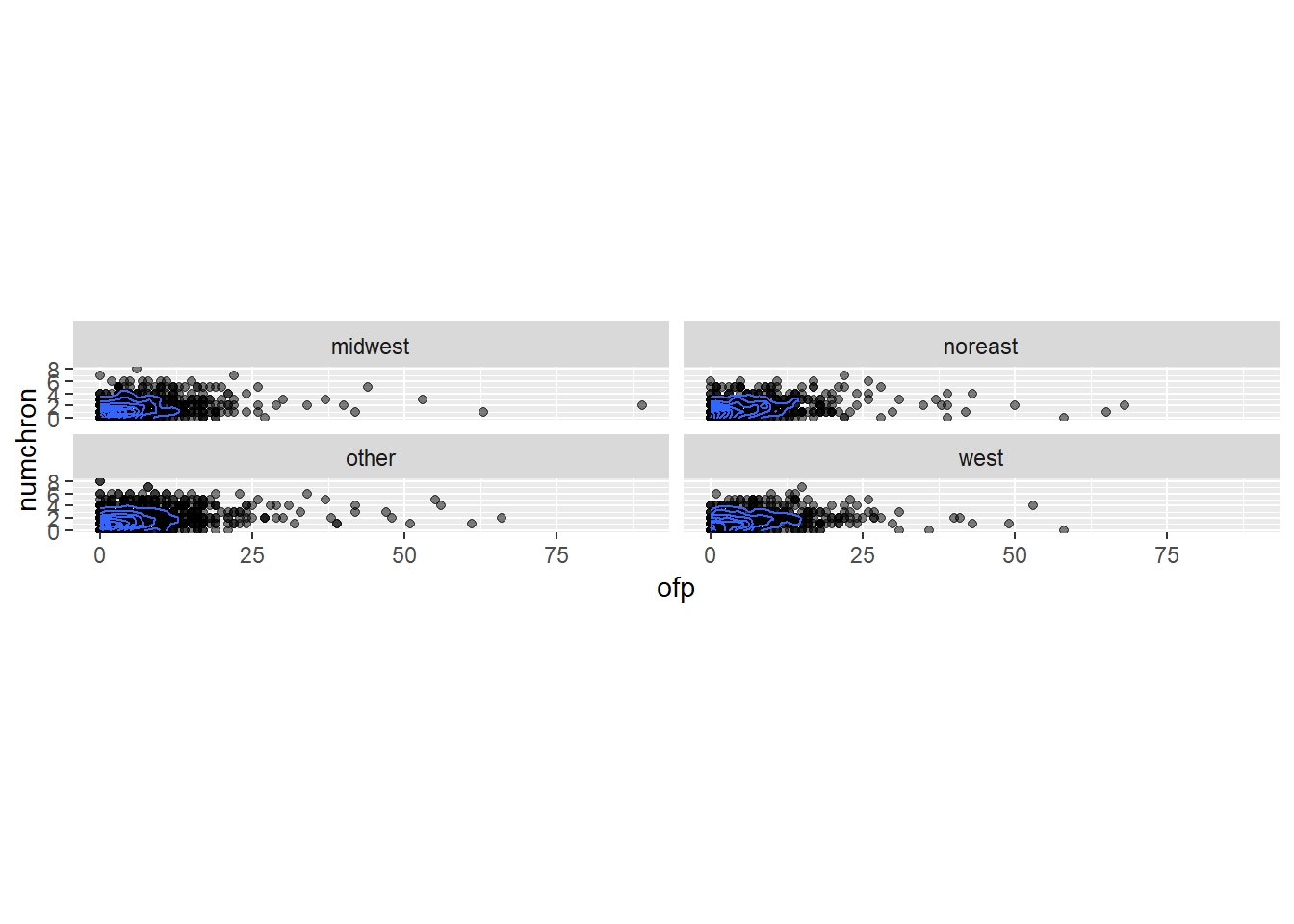
#Homogeneity
covmats<-visits%>%group_by(region)%>%do(covs=cov(.[2:3]))
for(i in 1:3){print(covmats$covs[i])}
## [[1]]
## ofp ofnp
## ofp 40.582725 6.319781
## ofnp 6.319781 37.474543
##
## [[1]]
## ofp ofnp
## ofp 54.43531 16.08302
## ofnp 16.08302 31.62989
##
## [[1]]
## ofp ofnp
## ofp 43.491422 5.260384
## ofnp 5.260384 16.457533#MANOVA
man1<-manova(cbind(ofp,opp,emr,hosp,numchron,age,school,faminc)~region, data=visits)
summary(man1)## Df Pillai approx F num Df den Df Pr(>F)
## region 3 0.044757 8.324 24 13191 < 2.2e-16 ***
## Residuals 4402
## ---
## Signif. codes: 0 '***' 0.001 '**' 0.01 '*' 0.05 '.' 0.1 ' ' 1#Univariate ANOVA
summary.aov(man1)## Response ofp :
## Df Sum Sq Mean Sq F value Pr(>F)
## region 3 583 194.286 4.262 0.005164 **
## Residuals 4402 200669 45.586
## ---
## Signif. codes: 0 '***' 0.001 '**' 0.01 '*' 0.05 '.' 0.1 ' ' 1
##
## Response opp :
## Df Sum Sq Mean Sq F value Pr(>F)
## region 3 3 1.136 0.0851 0.9682
## Residuals 4402 58771 13.351
##
## Response emr :
## Df Sum Sq Mean Sq F value Pr(>F)
## region 3 1.92 0.63973 1.2923 0.2752
## Residuals 4402 2179.15 0.49504
##
## Response hosp :
## Df Sum Sq Mean Sq F value Pr(>F)
## region 3 0.78 0.26003 0.4666 0.7056
## Residuals 4402 2453.29 0.55731
##
## Response numchron :
## Df Sum Sq Mean Sq F value Pr(>F)
## region 3 26.3 8.7558 4.8194 0.002368 **
## Residuals 4402 7997.5 1.8168
## ---
## Signif. codes: 0 '***' 0.001 '**' 0.01 '*' 0.05 '.' 0.1 ' ' 1
##
## Response age :
## Df Sum Sq Mean Sq F value Pr(>F)
## region 3 0.19 0.06341 0.1579 0.9246
## Residuals 4402 1767.10 0.40143
##
## Response school :
## Df Sum Sq Mean Sq F value Pr(>F)
## region 3 1941 647.07 47.766 < 2.2e-16 ***
## Residuals 4402 59633 13.55
## ---
## Signif. codes: 0 '***' 0.001 '**' 0.01 '*' 0.05 '.' 0.1 ' ' 1
##
## Response faminc :
## Df Sum Sq Mean Sq F value Pr(>F)
## region 3 507 169.017 20.016 6.989e-13 ***
## Residuals 4402 37171 8.444
## ---
## Signif. codes: 0 '***' 0.001 '**' 0.01 '*' 0.05 '.' 0.1 ' ' 1#t-tests
pairwise.t.test(visits$ofp,visits$region,
p.adj="none")##
## Pairwise comparisons using t tests with pooled SD
##
## data: visits$ofp and visits$region
##
## midwest noreast other
## noreast 0.0258 - -
## other 0.5152 0.0740 -
## west 0.0020 0.4080 0.0069
##
## P value adjustment method: nonepairwise.t.test(visits$opp,visits$region,
p.adj="none")##
## Pairwise comparisons using t tests with pooled SD
##
## data: visits$opp and visits$region
##
## midwest noreast other
## noreast 0.62 - -
## other 0.76 0.80 -
## west 0.87 0.76 0.92
##
## P value adjustment method: nonepairwise.t.test(visits$emr,visits$region,
p.adj="none")##
## Pairwise comparisons using t tests with pooled SD
##
## data: visits$emr and visits$region
##
## midwest noreast other
## noreast 0.647 - -
## other 0.076 0.264 -
## west 0.171 0.393 0.903
##
## P value adjustment method: nonepairwise.t.test(visits$hosp,visits$region,
p.adj="none")##
## Pairwise comparisons using t tests with pooled SD
##
## data: visits$hosp and visits$region
##
## midwest noreast other
## noreast 0.37 - -
## other 0.87 0.27 -
## west 0.87 0.33 0.98
##
## P value adjustment method: nonepairwise.t.test(visits$numchron,visits$region,
p.adj="none")##
## Pairwise comparisons using t tests with pooled SD
##
## data: visits$numchron and visits$region
##
## midwest noreast other
## noreast 0.64740 - -
## other 0.00053 0.00814 -
## west 0.36993 0.67854 0.03307
##
## P value adjustment method: nonepairwise.t.test(visits$age,visits$region,
p.adj="none")##
## Pairwise comparisons using t tests with pooled SD
##
## data: visits$age and visits$region
##
## midwest noreast other
## noreast 0.62 - -
## other 0.71 0.85 -
## west 0.89 0.56 0.64
##
## P value adjustment method: nonepairwise.t.test(visits$school,visits$region,
p.adj="none")##
## Pairwise comparisons using t tests with pooled SD
##
## data: visits$school and visits$region
##
## midwest noreast other
## noreast 0.65 - -
## other 7.2e-09 2.1e-06 -
## west 3.0e-10 3.5e-10 < 2e-16
##
## P value adjustment method: nonepairwise.t.test(visits$faminc,visits$region,
p.adj="none")##
## Pairwise comparisons using t tests with pooled SD
##
## data: visits$faminc and visits$region
##
## midwest noreast other
## noreast 0.2079 - -
## other 0.0019 3.4e-05 -
## west 6.7e-06 0.0024 5.0e-14
##
## P value adjustment method: none#bonferroni
1+8+48## [1] 570.05/57## [1] 0.000877193#Type I Error calc
1 - 0.95^57## [1] 0.9462665It is likely that independent observations were made but it isn’t known if this is a random sample. It might not be likely that homogeneity, multicollinearity, linear relationships among dependent variables and multivariance were met. I do not expect there to be extreme uni- or multivariaant outliers.
Assuming that the data passes the MANOVA assumptions, our hypothesis is that the numeric variables have equal means of the group for the categorical variable region. I left out the numeric variables number of nonphysician office visits and number of nonphysician outpatient visits because it would be redundant with number of physician office visits and number of physician outpatient visits included.
The MANOVA found that there is significantly different means among the numeric variables for region (p-value << 0.05). The bonferroni adjustment was made to control Type I error to correct alpha to 0.000877193 where from the follow up univariate ANOVA tests school and family income variables were found to have significantly mean difference across regions (p-value < 0.00088).
Post hoc analysis was done for pairwise comparisons of the significant variables to find what regions differed in number of years of school and family income. Only the midwest and north east regions not significantly differ in means for number of years in school. The midwest and west, other and north east, and west and other were the regions that significantly differed in family income. This analysis was done according to the bonferroni adjustment for multiple comparisons.
A total of 57 tests were done for this analysis (1 MANOVA, 8 ANOVA and 48 t-tests). There is a 0.9462 probability of at least one Type I error. The bonferroni test kept the error rate at 0.05 by adjusting to 0.00088 as discussed.
##Randomization Test
#null distribution
visits %>% ggplot(aes(faminc,fill=privins))+geom_histogram(bins=6.5)+facet_wrap(~privins) + xlab("Family Income ($10,000)") + ggtitle("Private Insurance for Family Incomes")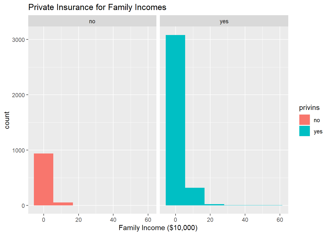
#mean diff
visits %>% group_by(privins) %>% summarize(means=mean(faminc)) %>% summarize(diff(means))
## # A tibble: 1 x 1
## `diff(means)`
## <dbl>
## 1 1.11#randomization
set.seed(348)
rand_dist<-vector()
for(i in 1:5000){
rand<-data.frame(income=sample(visits$faminc),insurance=visits$privins)
rand_dist[i]<-mean(rand[rand$insurance=="yes",]$income)-
mean(rand[rand$insurance=="no",]$income)}
#p-value
mean(rand_dist>1.112961)*2## [1] 0#t-test
t.test(data=visits,faminc~privins)##
## Welch Two Sample t-test
##
## data: faminc by privins
## t = -13.842, df = 2659.1, p-value < 2.2e-16
## alternative hypothesis: true difference in means is not equal to 0
## 95 percent confidence interval:
## -1.270625 -0.955296
## sample estimates:
## mean in group no mean in group yes
## 1.662984 2.775944{hist(rand_dist,main="Test Statistic Distribution",ylab="Frequency",xlim = c(-.4,1.2)); abline(v = 1.112961,col="red")}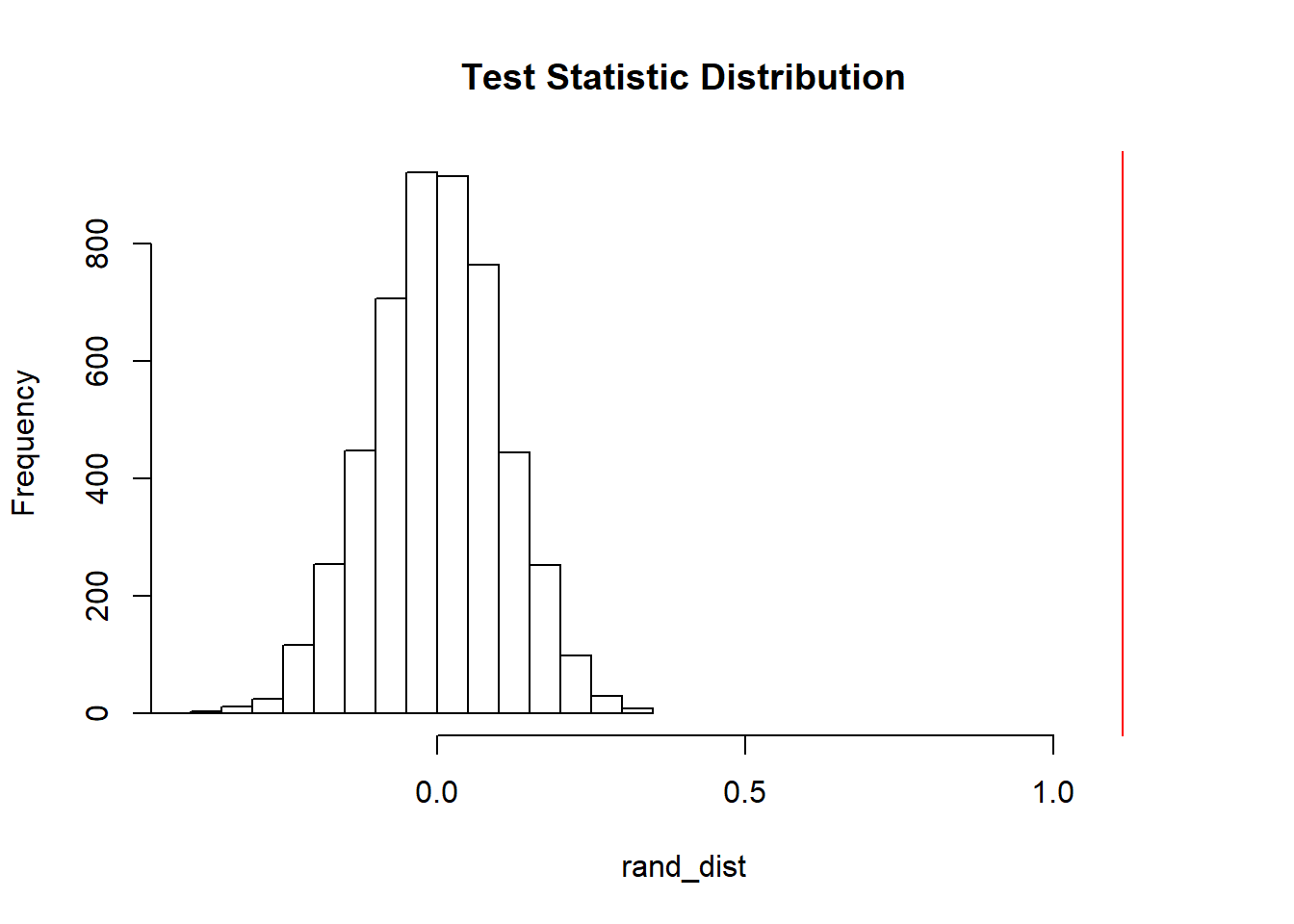 The null hypothesis for this randomization test is that mean family income is the same for
individuals with and without private insurance. The alternate hypothesis is that mean family income is different across individuals with and withouot private insurance.
##Linear Regression Model
#fit with interaction
visits$ofp_c<-visits$ofp-mean(visits$ofp)
visits$faminc_c<-visits$faminc-mean(visits$faminc)
fit <- lm(numchron ~ ofp_c*maried*faminc_c, data=visits)
summary(fit)
##
## Call:
## lm(formula = numchron ~ ofp_c * maried * faminc_c, data = visits)
##
## Residuals:
## Min 1Q Median 3Q Max
## -4.2727 -1.0343 -0.3119 0.6588 6.7424
##
## Coefficients:
## Estimate Std. Error t value Pr(>|t|)
## (Intercept) 1.589926 0.031457 50.543 <2e-16 ***
## ofp_c 0.046633 0.004478 10.414 <2e-16 ***
## mariedyes -0.066920 0.041479 -1.613 0.1067
## faminc_c 0.005960 0.014866 0.401 0.6885
## ofp_c:mariedyes 0.006964 0.006037 1.154 0.2487
## ofp_c:faminc_c -0.004273 0.001902 -2.246 0.0247 *
## mariedyes:faminc_c -0.031087 0.016807 -1.850 0.0644 .
## ofp_c:mariedyes:faminc_c 0.005468 0.002346 2.331 0.0198 *
## ---
## Signif. codes: 0 '***' 0.001 '**' 0.01 '*' 0.05 '.' 0.1 ' ' 1
##
## Residual standard error: 1.301 on 4398 degrees of freedom
## Multiple R-squared: 0.07292, Adjusted R-squared: 0.07144
## F-statistic: 49.42 on 7 and 4398 DF, p-value: < 2.2e-16#Plot
ggplot(visits, aes(x=ofp_c, y=numchron,group=maried))+geom_point(aes(color=maried))+
geom_smooth(method="lm",formula=y~1,se=F,fullrange=T,aes(color=maried))+xlab("Family Income ($10,000)") + ylab("Number of Chronic Illnesses") +ggtitle("Number of Chronic Illnesses by Family Income")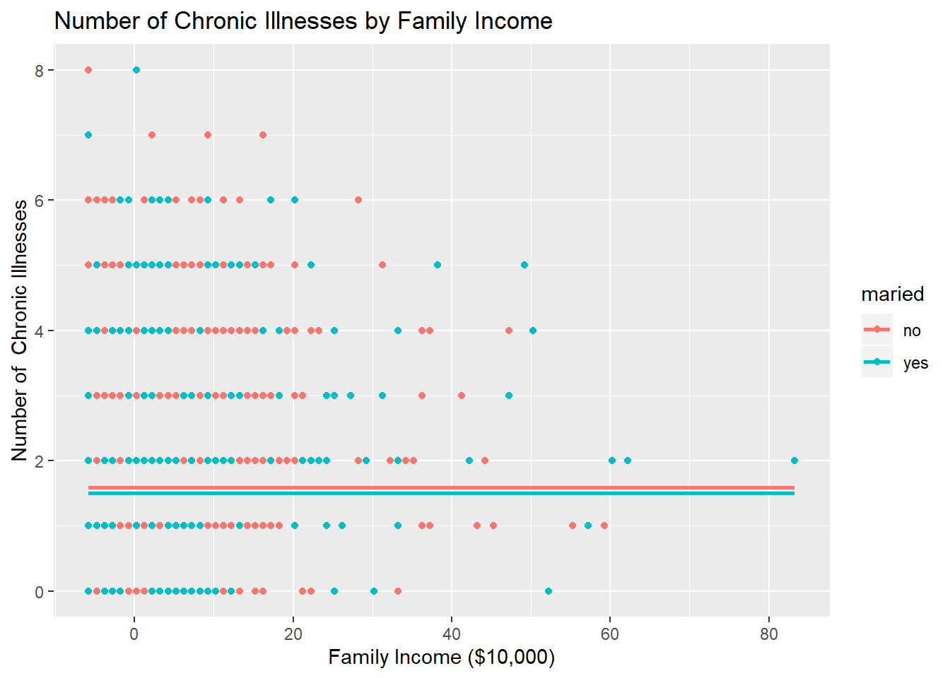
#Assumptions
resids<-fit$residuals; fitvals<-fit$fitted.values
ggplot()+geom_point(aes(fitvals,resids))+geom_hline(yintercept=0, col="red")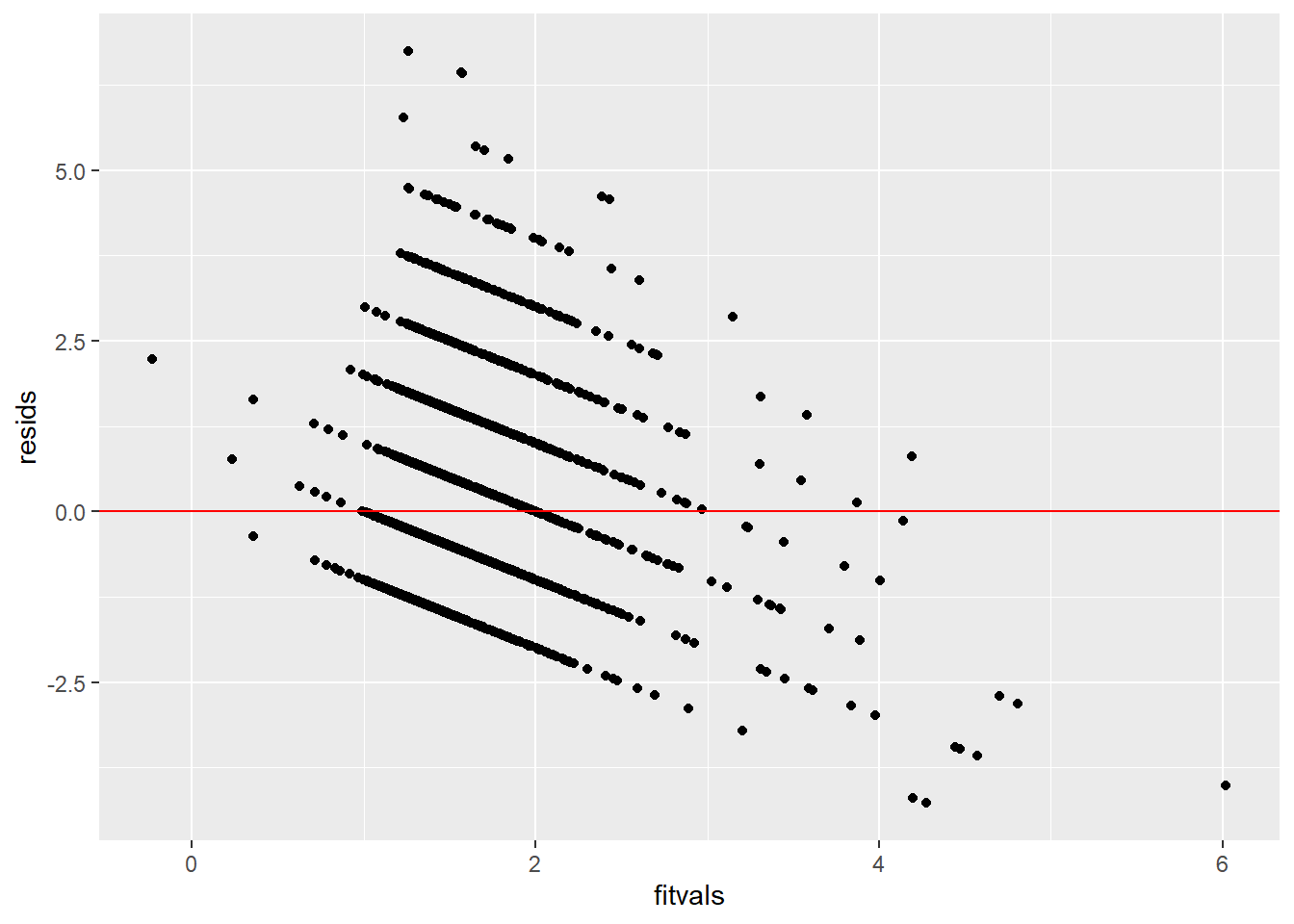
bptest(fit)##
## studentized Breusch-Pagan test
##
## data: fit
## BP = 120.01, df = 7, p-value < 2.2e-16ggplot()+geom_histogram(aes(resids),bins=20)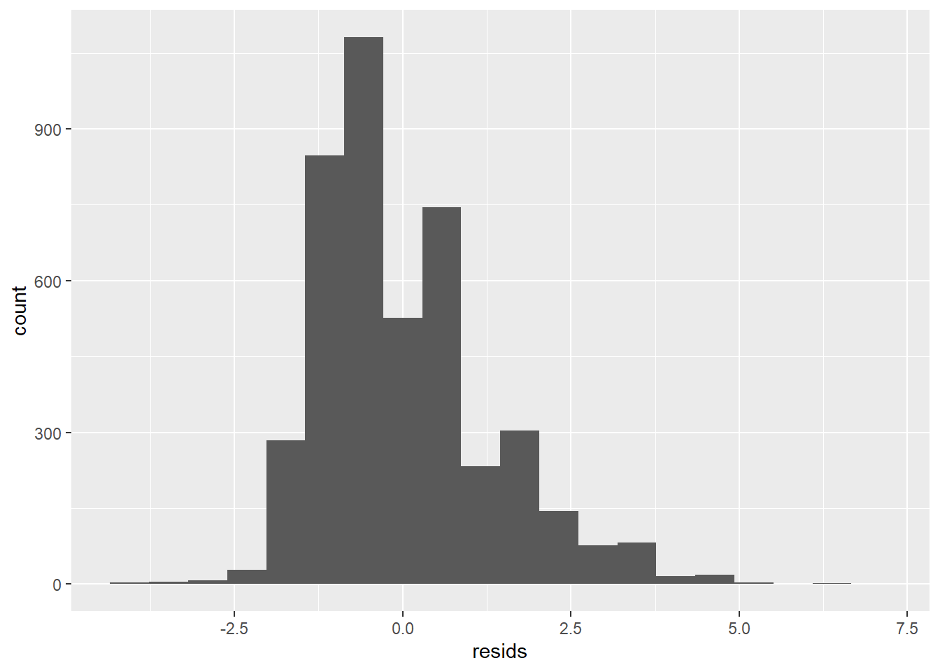
ggplot()+geom_qq(aes(sample=resids))+geom_qq_line()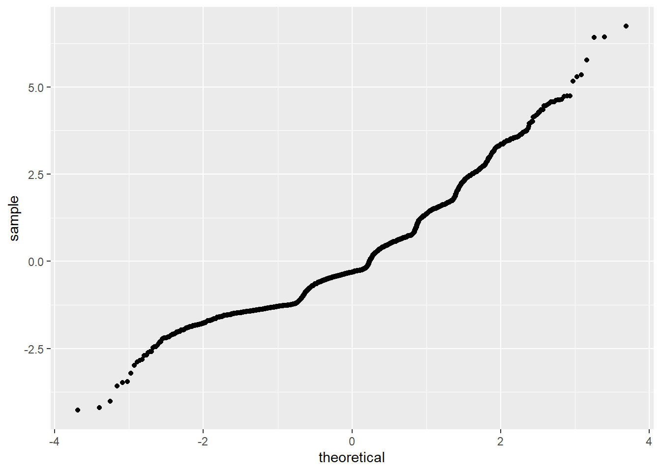
ks.test(resids, "pnorm", sd=sd(resids))## Warning in ks.test(resids, "pnorm", sd = sd(resids)): ties should not be
## present for the Kolmogorov-Smirnov test##
## One-sample Kolmogorov-Smirnov test
##
## data: resids
## D = 0.13155, p-value < 2.2e-16
## alternative hypothesis: two-sided#robust standard errors
summary(fit)$coef[,1:2]## Estimate Std. Error
## (Intercept) 1.589925786 0.031456758
## ofp_c 0.046633493 0.004477811
## mariedyes -0.066920123 0.041479153
## faminc_c 0.005960421 0.014865905
## ofp_c:mariedyes 0.006963694 0.006036566
## ofp_c:faminc_c -0.004272970 0.001902349
## mariedyes:faminc_c -0.031087335 0.016806799
## ofp_c:mariedyes:faminc_c 0.005467513 0.002345572coeftest(fit, vcov = vcovHC(fit))[,1:2]## Estimate Std. Error
## (Intercept) 1.589925786 0.033875220
## ofp_c 0.046633493 0.006720185
## mariedyes -0.066920123 0.043389741
## faminc_c 0.005960421 0.017991131
## ofp_c:mariedyes 0.006963694 0.009382407
## ofp_c:faminc_c -0.004272970 0.002789926
## mariedyes:faminc_c -0.031087335 0.020341280
## ofp_c:mariedyes:faminc_c 0.005467513 0.003488509#fit w/o interaction
fit2 <- lm(numchron ~ ofp_c+maried+faminc_c, data=visits)
summary(fit2)##
## Call:
## lm(formula = numchron ~ ofp_c + maried + faminc_c, data = visits)
##
## Residuals:
## Min 1Q Median 3Q Max
## -4.3095 -1.0708 -0.3061 0.6535 6.8883
##
## Coefficients:
## Estimate Std. Error t value Pr(>|t|)
## (Intercept) 1.569889 0.029633 52.977 < 2e-16 ***
## ofp_c 0.052171 0.002901 17.982 < 2e-16 ***
## mariedyes -0.051094 0.040695 -1.256 0.20935
## faminc_c -0.019085 0.006927 -2.755 0.00589 **
## ---
## Signif. codes: 0 '***' 0.001 '**' 0.01 '*' 0.05 '.' 0.1 ' ' 1
##
## Residual standard error: 1.301 on 4402 degrees of freedom
## Multiple R-squared: 0.07104, Adjusted R-squared: 0.07041
## F-statistic: 112.2 on 3 and 4402 DF, p-value: < 2.2e-16This linear regression used number of chronic illnesses as the response variable and mean centered physician’s office visits. marital status and family income as the predictors with interaction. The intercept, 1.59, is the predicted number of chronic illnessess when physician’s office visits and family income is 0 USD and unmarried. While holding marriage status and family income constant, for every 1 increase centered physician’s office visits the number of chronic illnesses is expected to increase by 0.0466. While holding physician’s office visits and family income constant, a married individudal will have 0.0669 less chronic illnesses than a person who isn’t married. While holding physician’s office visits and marital status constant, for every $1 increase in centered family income, the number of chronic illnessess will increase by 0.00596. The expected physicians office visits for non-married individuals is 0.006964 more than for those who are married. Family income is expected to be 0.0311 USD less for nonmarried people than married people. For each increase in physicians office vist, family income is expected to decrease by 0.004273 USD. For individuals who are not married, with each increase of physician’s office visits, family income is expected to increase 0.005458 USD more than for those who are married with each increase of physician’s office vists.
This data does not pass linearity, homoskedasticity, or normality.
Using robust standard error, the coefficients did not change. The SE’s increased with robust standard errors.
This model explains 7.292% of the variation in the outcome.
When running the model without interaction, one of the predictors (family income) is now significant.
##Bootstrapped Standard Errors of Linear Regression Model
samp_distn<-replicate(5000, {
 boot_dat<-boot_dat<-visits[sample(nrow(visits),replace=TRUE),]
 fit3<-lm(numchron ~ faminc_c * maried*ofp_c, data=boot_dat)
 coef(fit3)
})

samp_distn%>%t%>%as.data.frame%>%summarize_all(sd)
## (Intercept) faminc_c mariedyes ofp_c faminc_c:mariedyes
## 1 0.03338738 0.01741327 0.0427156 0.00653458 0.0195547
## faminc_c:ofp_c mariedyes:ofp_c faminc_c:mariedyes:ofp_c
## 1 0.002683802 0.009085953 0.003286179The bootstrapped standard errors are much more similar to the robust standard errors than the original, however they are slightly less. ##Logistic Regression
#regression
fit4<-glm(adldiff~ofp_c+faminc_c,data=visits,family=binomial(link="logit"))
coeftest(fit4)
##
## z test of coefficients:
##
## Estimate Std. Error z value Pr(>|z|)
## (Intercept) -1.4128048 0.0392614 -35.9846 < 2.2e-16 ***
## ofp_c 0.0352047 0.0050362 6.9904 2.741e-12 ***
## faminc_c -0.1358598 0.0204638 -6.6390 3.158e-11 ***
## ---
## Signif. codes: 0 '***' 0.001 '**' 0.01 '*' 0.05 '.' 0.1 ' ' 1exp(coef(fit4))## (Intercept) ofp_c faminc_c
## 0.2434595 1.0358317 0.8729650#confusion matrix
visits$prob<-predict(fit4,type="response")
table(predict=as.numeric(visits$prob>.5),truth=visits$adldiff)%>%addmargins## truth
## predict 0 1 Sum
## 0 3492 890 4382
## 1 15 9 24
## Sum 3507 899 4406#Accuracy
(3492+9)/4406## [1] 0.7945983#Sensitivity (TPR)
9/899## [1] 0.01001112#Specificity (TNR)
3492/3507## [1] 0.9957228#Recall (PPV)
9/24## [1] 0.375#plot
visits$logit<-predict(fit4) #get predicted log-odds
visits$outcome<-factor(visits$adldiff,levels=c("0","1"))
ggplot(visits,aes(logit, fill=outcome))+geom_density(alpha=.3)+
geom_vline(xintercept=0,lty=2)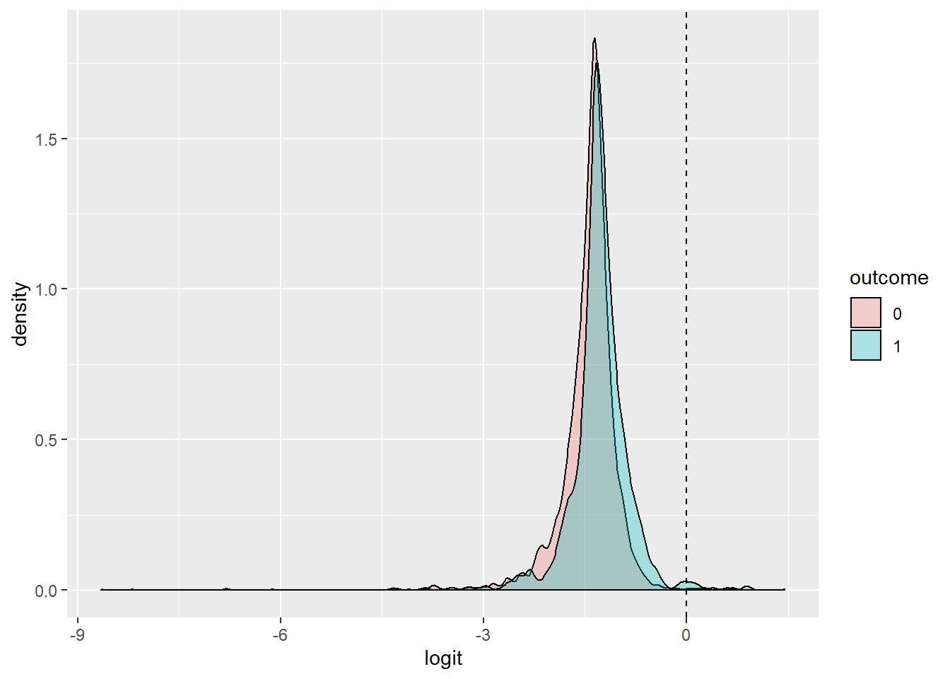
#ROC and AUC
ROCplot<-ggplot(visits)+geom_roc(aes(d=adldiff,m=prob), n.cuts=0)+
 geom_segment(aes(x=0,xend=1,y=0,yend=1),lty=2)
ROCplot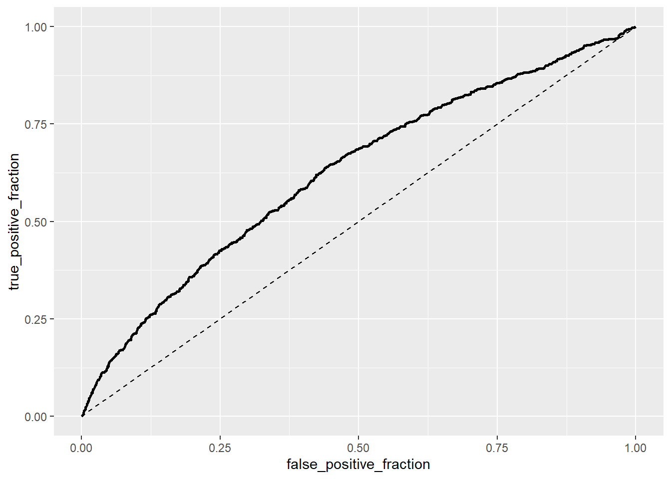
calc_auc(ROCplot)## PANEL group AUC
## 1 1 -1 0.6262655#function
class_diag<-function(probs,truth){
tab<-table(factor(probs>.5,levels=c("FALSE","TRUE")),truth)
acc=sum(diag(tab))/sum(tab)
sens=tab[2,2]/colSums(tab)[2]
spec=tab[1,1]/colSums(tab)[1]
ppv=tab[2,2]/rowSums(tab)[2]
if(is.numeric(truth)==FALSE & is.logical(truth)==FALSE) truth<-as.numeric(truth)-1
#CALCULATE EXACT AUC
ord<-order(probs, decreasing=TRUE)
probs <- probs[ord]; truth <- truth[ord]
TPR=cumsum(truth)/max(1,sum(truth))
FPR=cumsum(!truth)/max(1,sum(!truth))
dup<-c(probs[-1]>=probs[-length(probs)], FALSE)
TPR<-c(0,TPR[!dup],1); FPR<-c(0,FPR[!dup],1)
n <- length(TPR)
auc<- sum( ((TPR[-1]+TPR[-n])/2) * (FPR[-1]-FPR[-n]) )
data.frame(acc,sens,spec,ppv,auc)
}
#CV 10 fold
set.seed(1234)
k=10
visitscv<-visits[sample(nrow(visits)),]
folds<-cut(seq(1:nrow(visits)),breaks=k,labels=F)
diags<-NULL
for(i in 1:k){
train<-visitscv[folds!=i,]
test<-visitscv[folds==i,]
truth<-test$adldiff
fit5<-glm(adldiff~ofp+faminc,data=train,family="binomial")
probs<-predict(fit5,newdata = test,type="response")
diags<-rbind(diags,class_diag(probs,truth))
}
apply(diags,2,mean) ## acc sens spec ppv auc
## 0.794836116 0.008991227 0.996312405 NaN 0.625437875This logistic regression used the binary variable “adldiff” as the response variable and mean centered physician’s office visits and family income as predictors. When an individual has a family income of 0 and has never visited a physician’s office, their odds for having a condition limiting daily activity is 0.2801. While holding family income constant, odds of a condition limiting daily activity decreases 1.0358 with each increase in visit to a physician’s office. While holding physician office visits constant, each $10,000 increase in family income decreases the odds of a condition limiting daily activity by 0.1359. All predictors have a p-value less than 0.05, indicating the model is significant.
This model is about 79.46% accurate, however it is important to note, it has an extremely low true positive rate and near perfect true negative rate.
The AUC is close to 0.5, indicating that we can’t really predict individuals having a condition that limits their daily activity by family income and physicians office visits. ##Lasso Regression
visitslasso <- visits%>%dplyr::select(-prob,-outcome,-X,-logit)
y<-as.matrix(visitslasso$adldiff)
fit6 <- glm(adldiff~.-1, data = visitslasso, family = "binomial")
x<-model.matrix(fit6)
x<-scale(x)
cv<-cv.glmnet(x,y)
lasso1<-glmnet(x,y,lambda=cv$lambda.1se)
coef(lasso1)
## 25 x 1 sparse Matrix of class "dgCMatrix"
## s0
## (Intercept) 0.204039946
## ofp .
## ofnp .
## opp .
## opnp .
## emr 0.009571913
## hosp 0.001373959
## numchron 0.035682668
## age 0.082327961
## blackno .
## blackyes .
## sexmale -0.003289198
## mariedyes -0.009840636
## school -0.002073423
## faminc .
## employedyes .
## privinsyes .
## medicaidyes 0.034984107
## regionnoreast .
## regionother .
## regionwest .
## hlthother .
## hlthpoor 0.081731447
## ofp_c .
## faminc_c .#CV
set.seed(1234)
k=10
visitscv2<-visitslasso[sample(nrow(visitslasso)),]
folds<-cut(seq(1:nrow(visitslasso)),breaks=k,labels=F)
diags2<-NULL
for(i in 1:k){
train2<-visitscv2[folds!=i,]
test2<-visitscv2[folds==i,]
truth2<-test2$adldiff
fit7<-glm(adldiff~emr+hosp+numchron+age+sex+maried+school+medicaid+hlth,data=train2,family="binomial")
probs2<-predict(fit7,newdata = test2,type="response")
diags2<-rbind(diags2,class_diag(probs2,truth2))
}
diags2%>%summarize_all(mean)## acc sens spec ppv auc
## 1 0.8257045 0.3343958 0.9516561 0.6392141 0.8187942The LASSO regression shows that Emergency room visits, hospital visits, number of chronic illnesses, age, sex, marital status, years in school, medicaid coverage, and self reported health status to be the most important predictors of if an individual has a condition that limits their daily life. Running a 10 fold CV demonstrated a much higher AUC than from the model that only took into account family income and physician’s office visits.