January 1, 0001
library(tidyr)
library(ggplot2)
library(dplyr)
##
## Attaching package: 'dplyr'## The following objects are masked from 'package:stats':
##
## filter, lag## The following objects are masked from 'package:base':
##
## intersect, setdiff, setequal, unionIntroduction
The endorsements dataset is from https://projects.fivethirtyeight.com/2016-endorsement-primary/ and accounts for all of the endorsements of the 2016 primary election candidates based on a points system. Variables include the candidate, date, endorser, endorser’s position, and points the endorsement earned the candidate. The hiphop data set is from https://datahub.io/five-thirty-eight/hip-hop-candidate-lyrics#resource-genius_hip_hop_lyrics that compiles hip hop songs that reference the 2016 primary candidates. Variables include candidate, song, artist, sentiment, theme, album release date, the line of lyrics referencing the candidate, and url to lyrics.
These datasets interested me because I wanted to see if being referenced in a hip hop song had any correlation with endorsements for the 2016 primaries. The 2016 election was the first political event I was old enough to participate in and I remember it well. I expect to find that the more references in hiphop songs a candidate has, the more endorsements they will have. Likely if they are a big name, popular person they will be well established.
Tidying
endorsement <- read.csv("endorsement.csv")
endorsement %>% glimpse()
## Observations: 447
## Variables: 5
## $ ï..Candidate <fct> Hillary Clinton, Hillary Clinton, Hillary Clinton...
## $ Date <fct> 6/7/2016, 5/31/2019, 5/29/2019, 5/25/2019, 5/21/2...
## $ Endorser <fct> Nancy Pelosinew, Jerry Brownnew, Norma Torresnew,...
## $ Position <fct> Rep. (D-Calif.), Gov. (D-Calif.), Rep. (D-Calif.)...
## $ Pts. <int> 1, 10, 1, 5, 1, 1, 10, 1, 1, 1, 1, 1, 10, 1, 1, 1...hiphop <- read.csv("hiphop.csv")
hiphop %>% glimpse()## Observations: 377
## Variables: 9
## $ idz <int> 1, 2, 3, 4, 5, 6, 7, 8, 9, 10, 11, 12, 13, ...
## $ candidate <fct> Mike Huckabee, Mike Huckabee, Jeb Bush, Jeb...
## $ song <fct> none shall pass, wellstone, awe, the truth,...
## $ artist <fct> aesop rock, soul khan, dez & nobs, diabolic...
## $ sentiment <fct> neutral, negative, neutral, negative, negat...
## $ theme <fct> NA, NA, NA, political, personal, political,...
## $ album_release_date <int> 2011, 2012, 2006, 2006, 2007, 2012, 2001, 2...
## $ line <fct> "wither by the watering hole, border patrol...
## $ url <fct> http://genius.com/aesop-rock-none-shall-pas...colnames(endorsement)[1] <- "Candidate"
endorsement %>% na.omit() %>% glimpse()## Observations: 447
## Variables: 5
## $ Candidate <fct> Hillary Clinton, Hillary Clinton, Hillary Clinton, H...
## $ Date <fct> 6/7/2016, 5/31/2019, 5/29/2019, 5/25/2019, 5/21/2019...
## $ Endorser <fct> Nancy Pelosinew, Jerry Brownnew, Norma Torresnew, Ro...
## $ Position <fct> Rep. (D-Calif.), Gov. (D-Calif.), Rep. (D-Calif.), S...
## $ Pts. <int> 1, 10, 1, 5, 1, 1, 10, 1, 1, 1, 1, 1, 10, 1, 1, 1, 1...hh <- hiphop %>% na.omit() %>% glimpse()## Observations: 298
## Variables: 9
## $ idz <int> 4, 5, 6, 8, 9, 10, 11, 15, 18, 19, 21, 22, ...
## $ candidate <fct> Jeb Bush, Jeb Bush, Jeb Bush, Jeb Bush, Jeb...
## $ song <fct> the truth, money man, hidden agenda, bush s...
## $ artist <fct> diabolic, gorilla zoe, k-rino, macklemore, ...
## $ sentiment <fct> negative, negative, negative, negative, neg...
## $ theme <fct> political, personal, political, political, ...
## $ album_release_date <int> 2006, 2007, 2012, 2005, 2013, 2005, 2005, 2...
## $ line <fct> "what you heard before ain't as big of a le...
## $ url <fct> http://genius.com/diabolic-the-truth-lyrics...#already tidy so made untidy then pivoted from wide to long
endorsement %>% pivot_wider(names_from="Candidate", values_from="Date") %>% glimpse()## Observations: 407
## Variables: 21
## $ Endorser <fct> Nancy Pelosinew, Jerry Brownnew, Norma Torre...
## $ Position <fct> Rep. (D-Calif.), Gov. (D-Calif.), Rep. (D-Ca...
## $ Pts. <int> 1, 10, 1, 5, 1, 1, 10, 1, 1, 1, 1, 1, 10, 1,...
## $ `Hillary Clinton` <fct> 6/7/2016, 5/31/2019, 5/29/2019, 5/25/2019, 5...
## $ `Bernie Sanders` <fct> NA, NA, NA, NA, NA, NA, NA, NA, NA, NA, NA, ...
## $ `Joe Biden` <fct> NA, NA, NA, NA, NA, NA, NA, NA, NA, NA, NA, ...
## $ `Martin O'Malley` <fct> NA, NA, NA, NA, NA, NA, NA, NA, NA, NA, NA, ...
## $ `Donald Trump` <fct> NA, NA, NA, NA, NA, NA, NA, NA, NA, NA, NA, ...
## $ `Marco Rubio` <fct> NA, NA, NA, NA, NA, NA, NA, NA, NA, NA, NA, ...
## $ `Ted Cruz` <fct> NA, NA, NA, NA, NA, NA, NA, NA, NA, NA, NA, ...
## $ `John Kasich` <fct> NA, NA, NA, NA, NA, NA, NA, NA, NA, NA, NA, ...
## $ `Chris Christie` <fct> NA, NA, NA, NA, NA, NA, NA, NA, NA, NA, NA, ...
## $ `Jeb Bush` <fct> NA, NA, NA, NA, NA, NA, NA, NA, NA, NA, NA, ...
## $ `Mike Huckabee` <fct> NA, NA, NA, NA, NA, NA, NA, NA, NA, NA, NA, ...
## $ `Rand Paul` <fct> NA, NA, NA, NA, NA, NA, NA, NA, NA, NA, NA, ...
## $ `Lindsey Graham` <fct> NA, NA, NA, NA, NA, NA, NA, NA, NA, NA, NA, ...
## $ `Carly Fiorina` <fct> NA, NA, NA, NA, NA, NA, NA, NA, NA, NA, NA, ...
## $ `Ben Carson` <fct> NA, NA, NA, NA, NA, NA, NA, NA, NA, NA, NA, ...
## $ `Scott Walker` <fct> NA, NA, NA, NA, NA, NA, NA, NA, NA, NA, NA, ...
## $ `Rick Perry` <fct> NA, NA, NA, NA, NA, NA, NA, NA, NA, NA, NA, ...
## $ `Rick Santorum` <fct> NA, NA, NA, NA, NA, NA, NA, NA, NA, NA, NA, ...end <- endorsement %>% pivot_wider(names_from="Candidate", values_from="Date") %>%
pivot_longer(c("Hillary Clinton", "Bernie Sanders", "Joe Biden",
"Martin O'Malley", "Donald Trump", "Marco Rubio",
"Ted Cruz", "John Kasich", "Chris Christie", "Jeb Bush",
"Mike Huckabee", "Rand Paul", "Lindsey Graham",
"Carly Fiorina", "Ben Carson", "Scott Walker",
"Rick Perry", "Rick Santorum"), names_to="Candidate",
values_to="Date") %>% na.omit() %>% glimpse()## Observations: 447
## Variables: 5
## $ Endorser <fct> Nancy Pelosinew, Jerry Brownnew, Norma Torresnew, Ro...
## $ Position <fct> Rep. (D-Calif.), Gov. (D-Calif.), Rep. (D-Calif.), S...
## $ Pts. <int> 1, 10, 1, 5, 1, 1, 10, 1, 1, 1, 1, 1, 10, 1, 1, 1, 1...
## $ Candidate <chr> "Hillary Clinton", "Hillary Clinton", "Hillary Clint...
## $ Date <fct> 6/7/2016, 5/31/2019, 5/29/2019, 5/25/2019, 5/21/2019...NA’s were removed from the hiphop dataset. Under the theme’s variables there were about 79 rows that had a NA theme. Since these datasets were alreaady tidy, I untidied the endorsement dataset. I made it so that each candidate had their own column, with the date of endorsement as the values. I then retidied this from wide to long so that each date of endorsement had a row.
Joining/Merging
#creating number of endorsements variable
comb <- end %>% group_by(Candidate) %>% summarize(Endorsements=n_distinct(Endorser))%>%
  full_join(hh, by=c("Candidate"="candidate")) %>%
  distinct() %>% na.omit() %>% glimpse()
## Warning: Column `Candidate`/`candidate` joining character vector and
## factor, coercing into character vector## Observations: 296
## Variables: 10
## $ Candidate <chr> "Donald Trump", "Donald Trump", "Donald Tru...
## $ Endorsements <int> 15, 15, 15, 15, 15, 15, 15, 15, 15, 15, 15,...
## $ idz <int> 112, 114, 115, 116, 117, 118, 119, 120, 121...
## $ song <fct> protect ya neck ii the zoo, 50/banks, skill...
## $ artist <fct> 12 o'clock - brooklyn zu, 50 cent, nice, 69...
## $ sentiment <fct> positive, positive, positive, positive, pos...
## $ theme <fct> money, money, money, money, money, money, m...
## $ album_release_date <int> 1995, 2002, 1990, 1998, 2010, 1991, 1992, 1...
## $ line <fct> "given the power punch, soon to be paid lik...
## $ url <fct> http://genius.com/ol-dirty-bastard-protect-...#getting rid of unnecessary columns
comb2 <- comb %>% select(-idz,-url,-line) %>% glimpse()## Observations: 296
## Variables: 7
## $ Candidate <chr> "Donald Trump", "Donald Trump", "Donald Tru...
## $ Endorsements <int> 15, 15, 15, 15, 15, 15, 15, 15, 15, 15, 15,...
## $ song <fct> protect ya neck ii the zoo, 50/banks, skill...
## $ artist <fct> 12 o'clock - brooklyn zu, 50 cent, nice, 69...
## $ sentiment <fct> positive, positive, positive, positive, pos...
## $ theme <fct> money, money, money, money, money, money, m...
## $ album_release_date <int> 1995, 2002, 1990, 1998, 2010, 1991, 1992, 1...#creating number of song references variable
joined <- hh %>% group_by(candidate) %>% summarize(song_references=n_distinct(song))%>%
full_join(comb2, by=c("candidate"="Candidate")) %>%
na.omit() %>% glimpse()## Warning: Column `candidate`/`Candidate` joining factor and character
## vector, coercing into character vector## Observations: 296
## Variables: 8
## $ candidate <chr> "Donald Trump", "Donald Trump", "Donald Tru...
## $ song_references <int> 228, 228, 228, 228, 228, 228, 228, 228, 228...
## $ Endorsements <int> 15, 15, 15, 15, 15, 15, 15, 15, 15, 15, 15,...
## $ song <fct> protect ya neck ii the zoo, 50/banks, skill...
## $ artist <fct> 12 o'clock - brooklyn zu, 50 cent, nice, 69...
## $ sentiment <fct> positive, positive, positive, positive, pos...
## $ theme <fct> money, money, money, money, money, money, m...
## $ album_release_date <int> 1995, 2002, 1990, 1998, 2010, 1991, 1992, 1...First a new column was created that counted the number of endorseements each candidate had in 2016. A full join was done so that variables from both datasets could be compared. Unnecessaary columns idz, url to the song lyrics, and line of lyrics were dropped for the analysis. Then a variable for number of song references by each candidate was created.
##Wrangling
#summary 1: mean number of song references
joined %>% summarize(mean_song_references=mean(song_references))
## # A tibble: 1 x 1
## mean_song_references
## <dbl>
## 1 189.#summary 2: # of songs referencing Donald Trump
joined %>% filter(candidate=="Donald Trump") %>% group_by(candidate) %>%
summarize(donald_song_references=n_distinct(song)) %>%
glimpse()## Observations: 1
## Variables: 2
## $ candidate <chr> "Donald Trump"
## $ donald_song_references <int> 228#summary 3 mean album release date
joined %>% na.omit() %>% summarize(mean_album_date=mean(album_release_date))## # A tibble: 1 x 1
## mean_album_date
## <dbl>
## 1 2008.#summary 4 group by candidate, minimum endorsements
joined %>% group_by(candidate) %>% summarize(least_endorsements=min(Endorsements)) %>%
arrange(least_endorsements)## # A tibble: 4 x 2
## candidate least_endorsements
## <chr> <int>
## 1 Donald Trump 15
## 2 Jeb Bush 31
## 3 Ted Cruz 44
## 4 Hillary Clinton 225#summary 5 candidate referencing songs in 2015 and 2016
joined %>% select(candidate, song, album_release_date) %>%
arrange(album_release_date) %>%
filter(album_release_date==2015 | album_release_date==2016) ## # A tibble: 50 x 3
## candidate song album_release_date
## <chr> <fct> <int>
## 1 Donald Trump planewalker 2015
## 2 Donald Trump neighborhood scientists 2015
## 3 Donald Trump up like trump 2015
## 4 Donald Trump pnt 2015
## 5 Donald Trump she wanna fuck 2015
## 6 Donald Trump dope spot 2015
## 7 Donald Trump florida state 2015
## 8 Donald Trump have a nice day 2015
## 9 Donald Trump flavas back 2015
## 10 Donald Trump 10 times 2015
## # ... with 40 more rowsjoined %>% select(candidate, song, album_release_date) %>%
arrange(album_release_date) %>%
filter(album_release_date==2015 | album_release_date==2016) %>%
group_by(album_release_date) %>%
summarize(count=n()) ## # A tibble: 2 x 2
## album_release_date count
## <int> <int>
## 1 2015 30
## 2 2016 20#summary 6 number of times artists referenced candidates
joined %>% select(artist, candidate) %>% group_by(artist) %>%
summarize(artist_cand_ref=n()) %>% arrange(artist) %>%
glimpse()## Observations: 216
## Variables: 2
## $ artist <fct> 12 o'clock - brooklyn zu, 2 chainz, 50 cent, 6...
## $ artist_cand_ref <int> 1, 1, 2, 1, 1, 1, 1, 1, 1, 1, 1, 1, 1, 1, 2, 1...#summary 7 song references to endorsements proportion
joined %>% mutate(proportion=song_references/Endorsements) %>%
summarize(proportion_sd=sd(proportion))## # A tibble: 1 x 1
## proportion_sd
## <dbl>
## 1 6.23#summary 8 distinct sentiments/how many positive, neutral, negative
joined %>% group_by(candidate,sentiment) %>% summarize(n=n()) %>%
spread(sentiment,n, fill=0)## # A tibble: 4 x 4
## # Groups: candidate [4]
## candidate negative neutral positive
## <chr> <dbl> <dbl> <dbl>
## 1 Donald Trump 24 51 155
## 2 Hillary Clinton 22 25 11
## 3 Jeb Bush 5 2 0
## 4 Ted Cruz 1 0 0#summary 9 group/arrange by song distinct themes/how many personal, political, etc. by sentiment
joined %>% group_by(theme,sentiment) %>% summarize(n=n()) %>% spread(theme,n, fill=0)## # A tibble: 3 x 8
## sentiment hotel money personal political power sexual `the apprentice`
## <fct> <dbl> <dbl> <dbl> <dbl> <dbl> <dbl> <dbl>
## 1 negative 0 1 13 36 0 2 0
## 2 neutral 7 15 25 10 1 2 18
## 3 positive 61 91 9 4 1 0 0#summary 10 correlation number of songs per candidate and number of endorsements per candidate
joined %>% select_if(is.numeric)%>%na.omit%>%cor## song_references Endorsements album_release_date
## song_references 1.00000000 -0.89030810 0.07930277
## Endorsements -0.89030810 1.00000000 -0.09045409
## album_release_date 0.07930277 -0.09045409 1.00000000Basic summary statistics were taken from the joined data to find the mean number of song references for a candidate, the number of songs referencing Donald Trump who went on to win the 2016 election, the mean album release date, which actually is 8 years before the election took place, and finally the lowest number of candidate endorsements. Primaries began in 2015 when endorsements first were being made so a count of songs released in 2015 and 2016 were taken in order to find if there was any effect with endorsements.
Then a count of how many times each artist referenced a candidate was made. Jay Z referenced 2016 candidates in 4 songs. A standard deviation of the proportion of song references to endorsements for candidates was caluclated to be 6.233. Out of song references, a spread was created by each candidate for the sentiment of the song they were referenced in which includes the options of negative, neutral, and positive. To follow that statistic, the theme of each sentiment was spread to cover hotel, money, personal, political, power, sexual, and The Apprentice. Finally a correlation of numeric variables was calculated. Unexpectedly, there is a negative correlation between endorsement and song references while album release date has no correlation to endorsements.
Visualizing
#plot 1: candidate, sentiment
ggplot(joined, aes(candidate, Endorsements)) + geom_bar(stat="summary", fun.y="mean", fill="#faf5c3") +
  geom_point(aes(candidate, song_references, color=song_references)) +
  scale_color_gradient(low="blue", high="orange") +
  ggtitle('Candidate Song References & Endorsements') +
  xlab('Candidate') + ylab('Number Of Endorsements') +
  scale_y_continuous(lim=c(0,300),
                     breaks=c(0,25,50,75,100,125,150,175,200,225,250,275,300))
#plot 2: candidate, theme, sentiment, album release date
ggplot(joined, aes(sentiment, album_release_date)) + geom_point(aes(color=theme), size=.5) +
  facet_wrap(~candidate) + theme_dark() +
  ggtitle('Themes & Sentiments of Candidates Referenced In Songs by Year')+
  xlab('Sentiment') + ylab('Album Release Date') +
  scale_y_continuous(lim=c(1989,2016),
                     breaks=c(1989,1991,1993,1995,1997,1999,2001,
                              2003,2005,2007,2009,2011,2013, 2015))
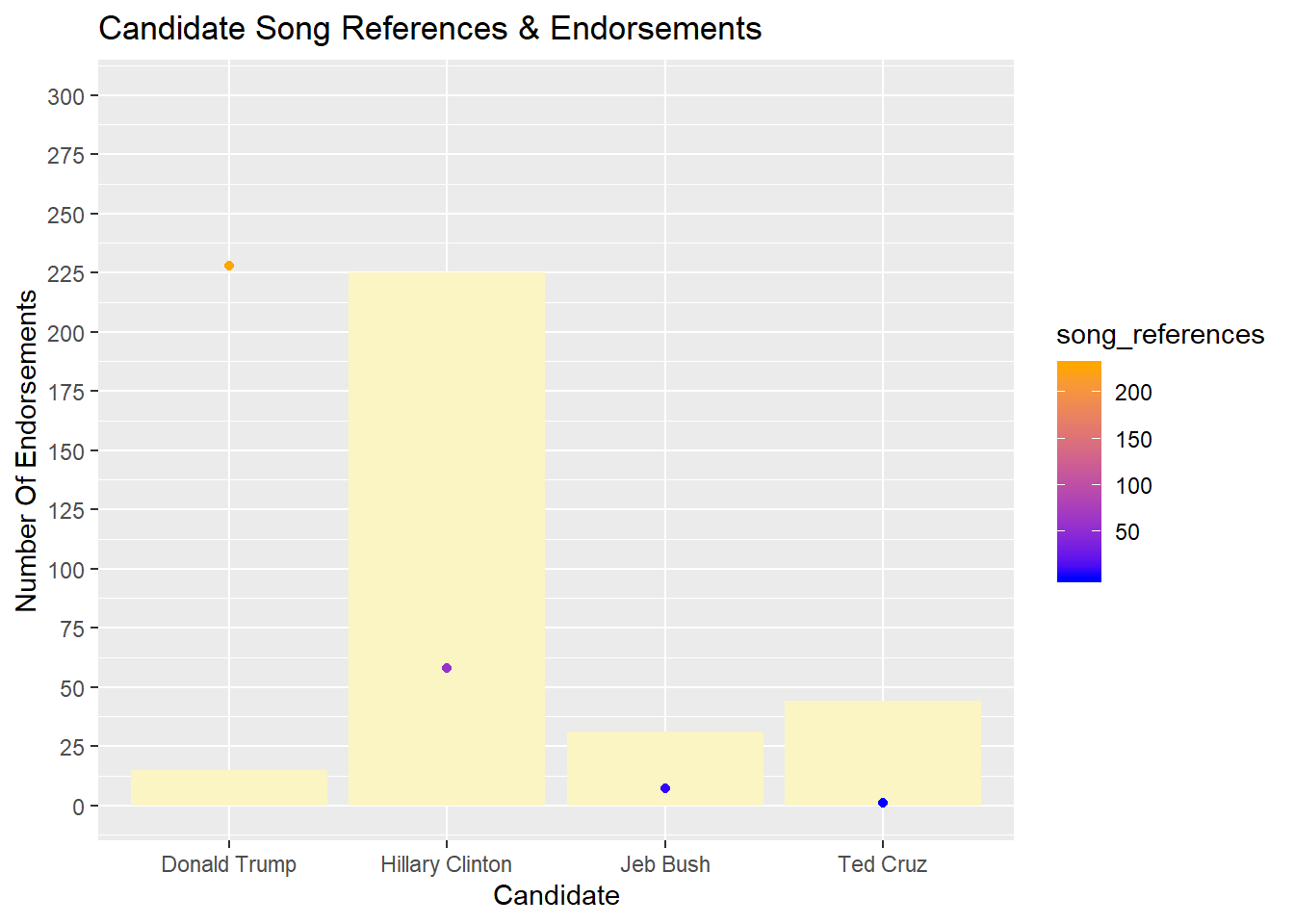
The first plot demonstrates how many endorsements and song references each candidate had up to the 2016 election.
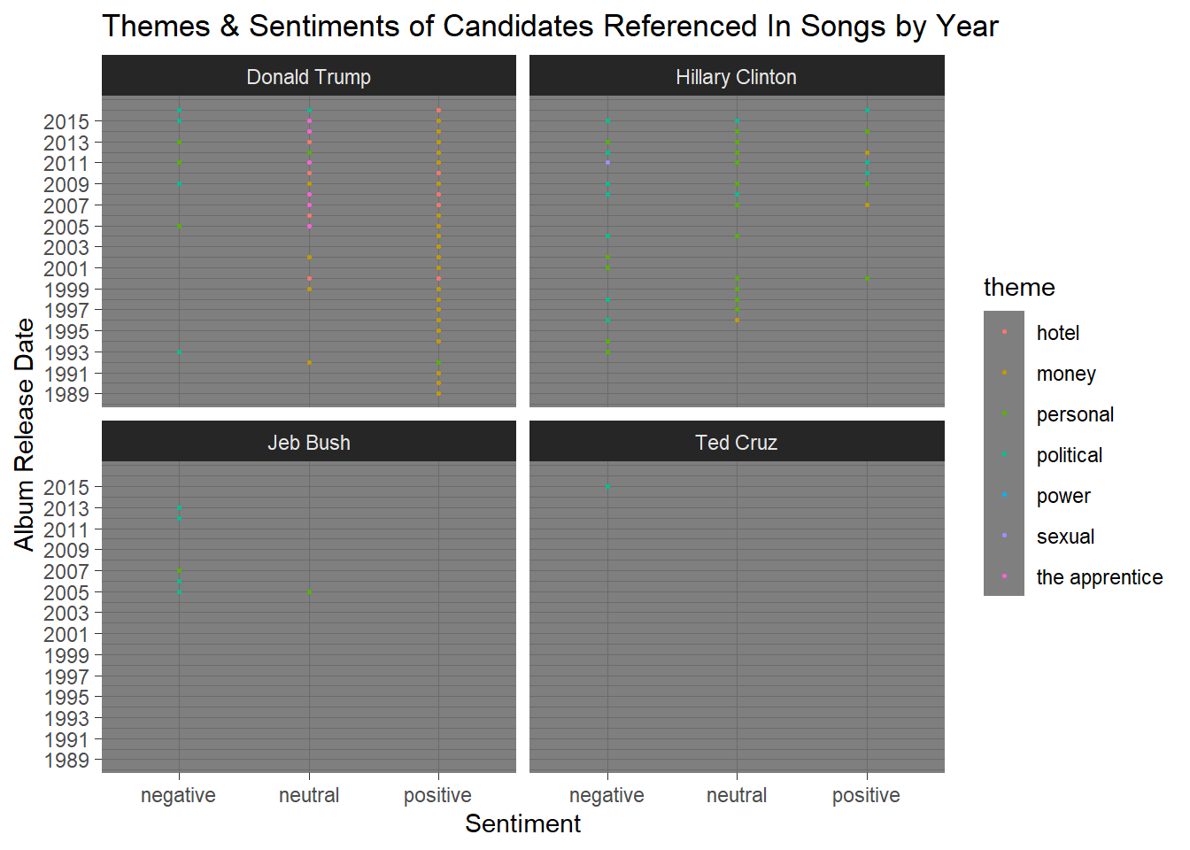
The second plot compares the sentiments and themes of candidates referenced in songs by the year the album was released.
Dimensionality Reduction
#covariance
joined%>%select_if(is.numeric)%>%cov
## song_references Endorsements album_release_date
## song_references 5465.60215 -5483.6263 39.74114
## Endorsements -5483.62627 6940.9199 -51.08220
## album_release_date 39.74114 -51.0822 45.94792#scale
joined_num<-joined%>%select_if(is.numeric)%>%scale %>% glimpse()## num [1:296, 1:3] 0.532 0.532 0.532 0.532 0.532 ...
## - attr(*, "dimnames")=List of 2
## ..$ : NULL
## ..$ : chr [1:3] "song_references" "Endorsements" "album_release_date"
## - attr(*, "scaled:center")= Named num [1:3] 188.7 56.6 2008.2
## ..- attr(*, "names")= chr [1:3] "song_references" "Endorsements" "album_release_date"
## - attr(*, "scaled:scale")= Named num [1:3] 73.93 83.31 6.78
## ..- attr(*, "names")= chr [1:3] "song_references" "Endorsements" "album_release_date"joined_pca<-princomp(joined_num)
names(joined_pca)## [1] "sdev" "loadings" "center" "scale" "n.obs" "scores"
## [7] "call"summary(joined_pca, loadings=T)## Importance of components:
## Comp.1 Comp.2 Comp.3
## Standard deviation 1.3783210 0.9903762 0.33053152
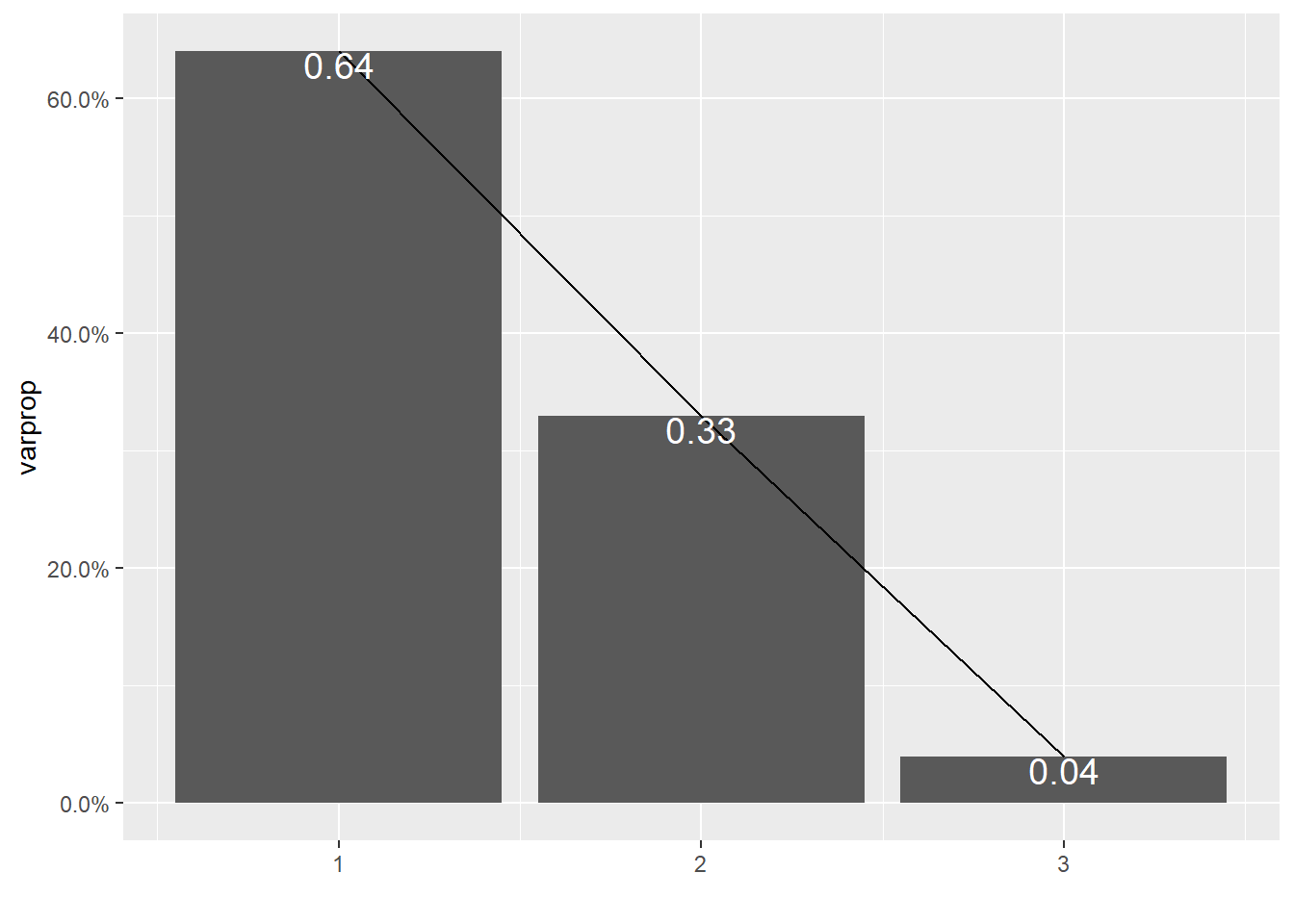
## Proportion of Variance 0.6354029 0.3280566 0.03654048
## Cumulative Proportion 0.6354029 0.9634595 1.00000000
##
## Loadings:
## Comp.1 Comp.2 Comp.3
## song_references 0.701 0.707
## Endorsements -0.701 0.708
## album_release_date 0.131 -0.991eigval<-joined_pca$sdev^2
varprop=round(eigval/sum(eigval),2)
ggplot()+geom_bar(aes(y=varprop,x=1:3),stat="identity")+xlab("")+geom_path(aes(y=varprop,x=1:3))+
geom_text(aes(x=1:3,y=varprop,label=round(varprop,2)),vjust=1,col="white",size=5)+
scale_y_continuous(breaks=seq(0,.6,.2),labels = scales::percent)+
scale_x_continuous(breaks=1:13)
eigvalround<-round(cumsum(eigval)/sum(eigval),2)
eigvalround
## Comp.1 Comp.2 Comp.3
## 0.64 0.96 1.00summary(joined_pca, loadings=T)## Importance of components:
## Comp.1 Comp.2 Comp.3
## Standard deviation 1.3783210 0.9903762 0.33053152
## Proportion of Variance 0.6354029 0.3280566 0.03654048
## Cumulative Proportion 0.6354029 0.9634595 1.00000000
##
## Loadings:
## Comp.1 Comp.2 Comp.3
## song_references 0.701 0.707
## Endorsements -0.701 0.708
## album_release_date 0.131 -0.991joineddf<-data.frame(PC1=joined_pca$scores[,1], PC2=joined_pca$scores[,2])
ggplot(joineddf,aes(PC1, PC2))+geom_point()
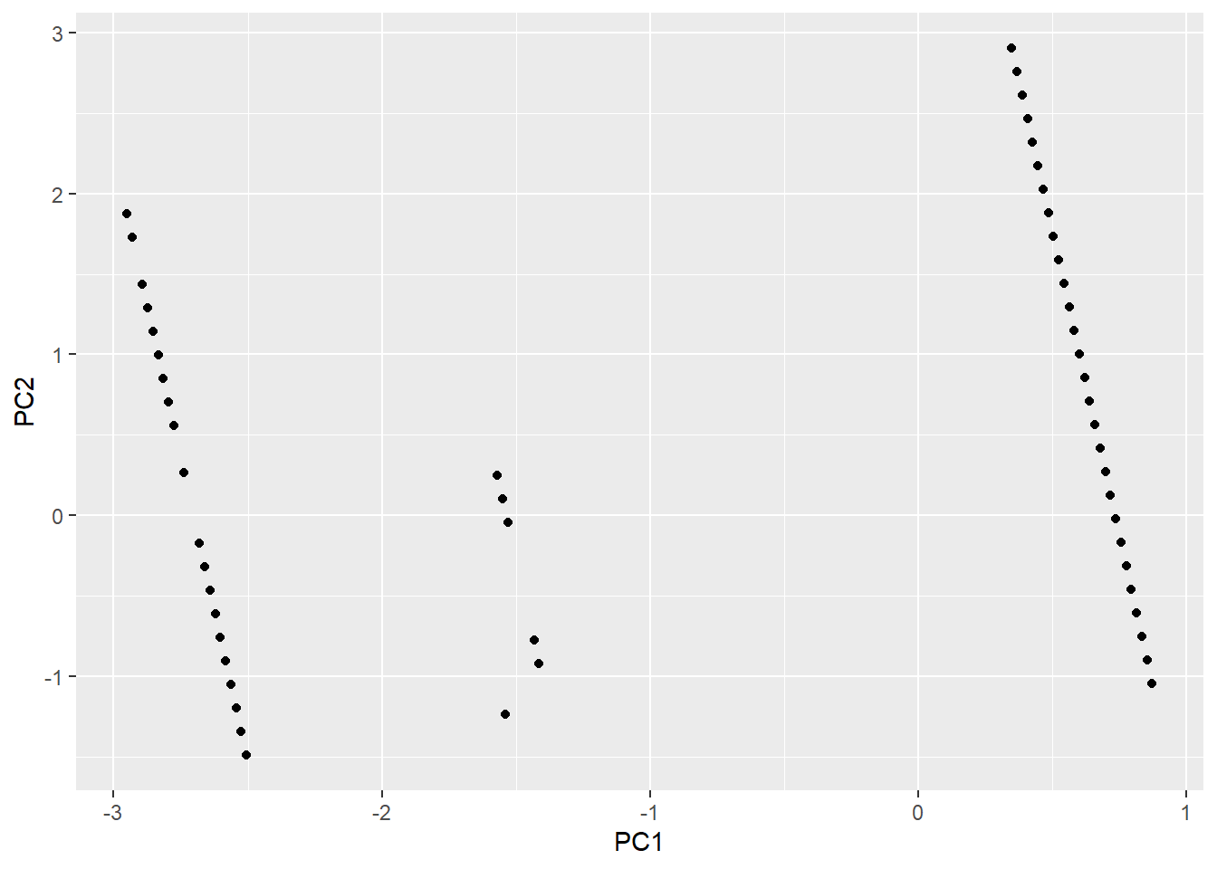
There is a high negative covariance between endorsements and song references meaning that they don’t distinguish observations from each other. PC1 does not have much similarity. Album release date has very different magnitude from song references and endorsements, but has same sign as song references. Song references and endorsements have very similar magnitudes but opposite signs. PC2 is song references vs endorsements axis, where album release date is high scoring. PC3 is an axis for album release date where endorsements and song references have near magnitude and sign.
In the plot of loadings, each principal component appears to only be associated with one variable each. There are large angles between vectors implyng a low correlation. Therefore this study can conclude that there is not a significant correlation between song references on endorsements.